Productivity : useful and dark corners of Excel

Everybody knows Excel. The world’s leading spreadsheet application. but do we really use it to do just spread-sheets editing or can we do more with it?

Excel could be used to Automate tasks, to analyze data and go beyond just creating reports.

In this article I try to expose some of the functionalities I mostly use in Excel as developer and production support staff at the same time.

Before we start:

Before we go ahead, you need to be aware of some terminologies in order to make the reading of this article easier.

• An Excel WORKBOOK has multiple WORKSHEETS in it.
• Each WORKSHEET is composed of multiple CELLS and they are described by row and column.
• ROW  names are  Numerals and COLUMN names are Alphabet. In order to describe a CELL you need to define COLUMN-ROW example “A1”.
• A RANGE is a group of   CELLS.
• A range could be defined by the upper left cell and lower right cell example “A1:C6”.
• A RANGE could be named pressing F5 to assign an arbitrary name to the range.

Pivot Tables.

If you have a table with repeating data, and you need to generate aggregate views of the data, Pivot tables is your man for the job. Or lets just say that is one of its many uses. It can help you group and sub-group data. It can also help you catch a thief, detect fraud and save world peace if you really know how to use it.

Ok let us get series, I think I went really too far with the world peace thingy, but really it is helpful if you are looking inside large amounts of data or if you are looking for patterns inside your data.

I always believed that the best way to explain things is by telling a story, or as we in IT like to call them Scenarios:

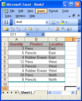
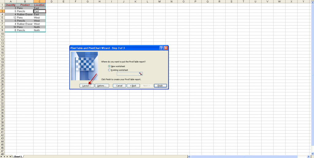
Imagine you have a long table of stationary sales data:

Of course you have to assume that the data is much more than this. but we are using a small sample for simplicity.

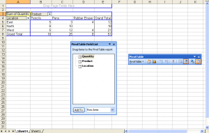
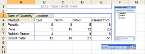
With Pivot tables you can convert that data into something like this:

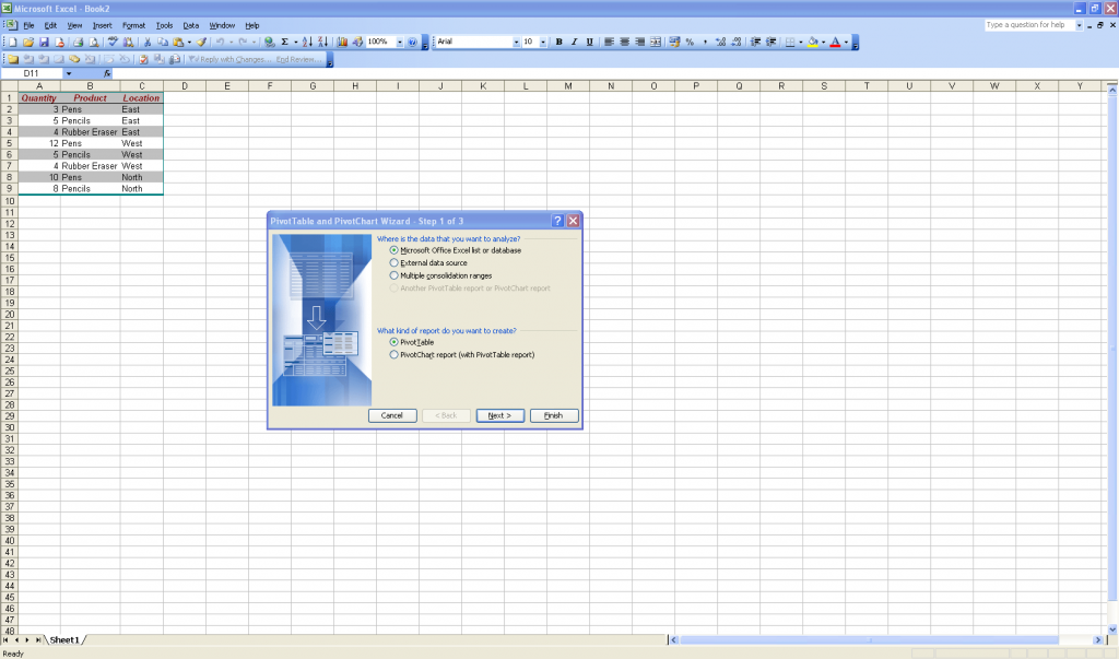
To get to this final result we followed these steps:

1. Click inside the table you want to pivot:
   

   Click inside the table and from the menu bar "Data->Pivot Table and .."

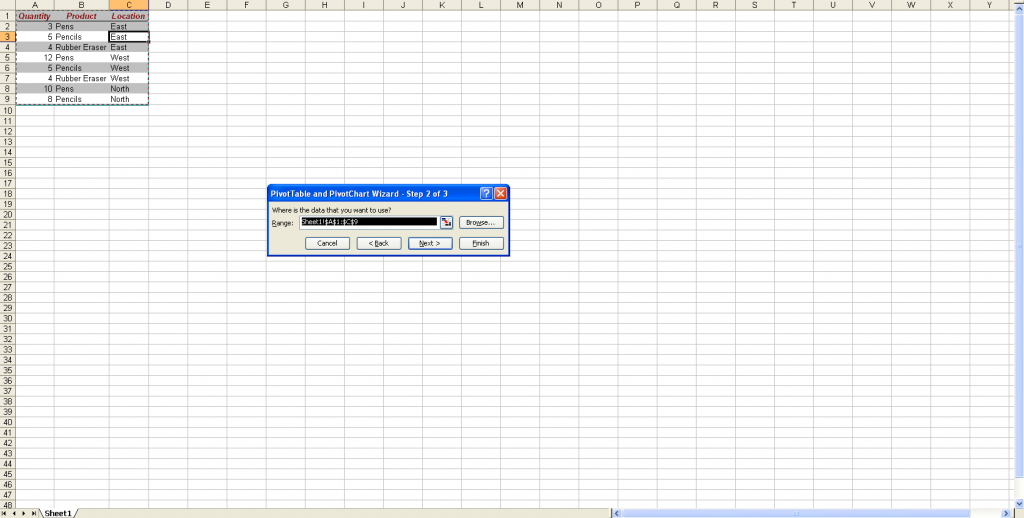
2. Verify the range you want to generate the Pivot table for:
   

   Verify the selected range to be true

3. 

   Click the layout button

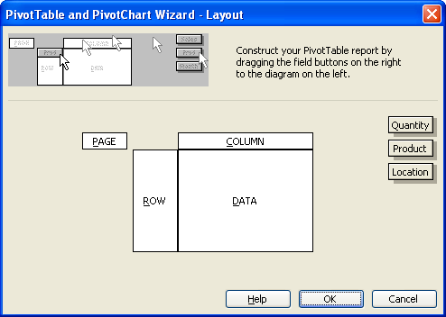
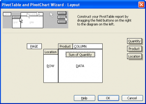
4. you will get a window like this, with the Column Headers identified. Drag the Columns and drop them as indicated:
   

   drag the column headers into the Column, data and row

   

   notice the data sections mentions "SUM OF ..." , this could be changed by double clicking into Avg,Count,....etc

5. Finally you get the result as indicated below:

 

 

 

This feature could be used to create marvelous Executive and summary reports. sort of show the trees in the forest reports. You could manipulate the PIVOT table by right-clicking and then “Pivot table wizard” then click the “Layout” button.

VLOOKUP

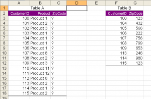
You have two tables, tables A and B , some records in Table A are also in table B. you need to find out where tables A and B intersect. or sometimes also, Table A has some extra data or column which is not in list B or vice versa. VLOOKUP Excel function could be used to match the records per one Primary key column and fetch the missing data from table A to B.

The general syntax of the VLOOKUP worksheet function:

VLOOKUP(lookup_value,table_array,col_index_num,range_lookup)

VLOOKUP: Searches for a value in the leftmost column of a table, and then returns a value in the same row from a column you specify in the table.

 

1. You have to decide what is the Key you will use to LOOKUP inside the two lists. In this case it is CustomerID.
2. You have to Sort both lists based on the the Key chosen in step1.
   

   Sorting

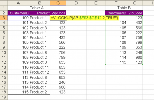
3. Go to cell C:3 and type the following: =VLOOKUP(A3;$F$3:$G$12;2;TRUE) this will search the area F3:G12 (a ranges of cells) for the value that is in cell A3, and will match it to the cells in the Columns F3:F12 (as per the search tables) and fetch the Values in the 2nd Column after F which is G column. and if no matching value is found it will take the Closest Customer ID. We Marked the lookup table range with $ (dollar sign) to prevent excel from changing the Lookup table range while dragging the function downwards. (sort of a fixed range).
   

   VLOOKUP with TRUE option

    

4. If VLOOKUP can’t find lookup_value, and range_lookup is TRUE, it uses the largest value that is less than or equal to lookup_value.
5. If lookup_value is smaller than the smallest value in the first column of table_array, VLOOKUP returns the #N/A error value.
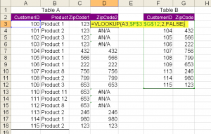
6. If VLOOKUP can’t find lookup_value, and range_lookup is FALSE, VLOOKUP returns the #N/A value.
   

   VLOOKUP with FALSE option

The Microsoft help is very rich with information ( just go to any cell and type “=vlookup(” and press F1).

Also a related sister function -but less frequently used- HLOOKUP() could be used to do the same in case te primary key is Horizontal.

Find Duplicates in list:

There are many ways to find duplicates in list or a column, simplest is:

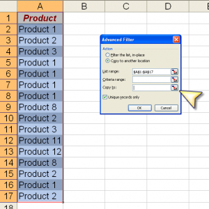
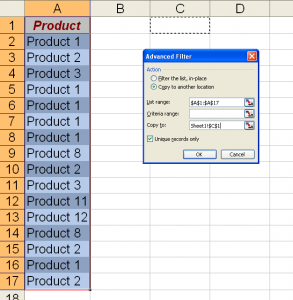
DATA-> Filter -> Advanced Filter

Click “Unique records Only” and “Copy to another location” then click as shown above to determine where the new list will show.

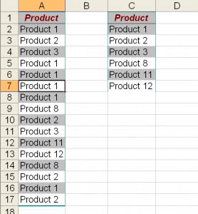
The resulting unique list:

you could also use PIVOT tables feature to find out duplicates and even their frequency.

Web Query

I haven’t used this feature so much; but I could assume it is useful if you keep querying data from the web and using it inside Excel.

It is a feature that helps fetch HTML tables into Excel for further processing. Things like following up on Stock prices and Exchange rates could benefit greatly from such a feature.

There is enough material on the web, just search for “Excel Web Query”.

External Queries

Very useful if you need to create dashboard based on DATABASE input. you could use SQL to select data and convert it into Pivot table or chart on the spot, you could even adjust a refresh period, in case you are watching live data.

1- For Excel to be able to read various types of data-source, it needs to use ODBC. To define a new data-source, go to “Control Panel” then “Administrative Tools” and then click the icon “Data Sources (ODBC) “. choose “User DSN” or “System DSN” and click “Add” button. insert there the credentials like database name , user name and password. Then “Test Connection” in case everything is fine continue to the next paragraph.

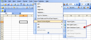
2- Once an ODBC data source has been defined, go to excel and click where you want to insert your data. Then go to the menu and chose “Data->Import External Data->New Database Query “. If you are familiar with Access, you will know what to do later. You can chose the tables and columns decoratively or you can type in your SQL statement.

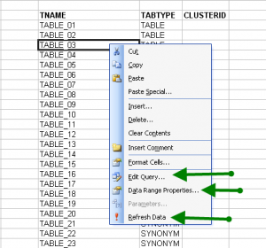
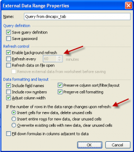
3- once the external query runs and data is fetched back from Microsoft Query back to Excel sheet.  You have multiple options available for you to chose from. you can Trigger another refresh of the data manually , alter the properties of the data range like SQL or shown columns or make the query Auto refreshing every x seconds like the dialog box below:

Please don’t get any funny ideas about using this feature to update your database tables through Excel. It is not supported.

If  you format the data-range with colors and font adjustments, every refresh will maintain your formatting unless you adjust it otherwise.

Another alternative to this feature is to use VBA to fetch and inject the data into your sheet.

This feature is quit useful if you are generating KPI’s from a database or following up on a running database activity… etc.

Split Data Columns

There are two scenarios when you need this feature:

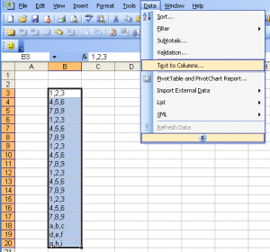
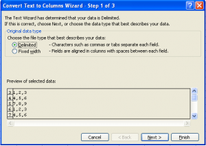
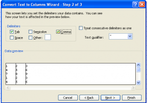
1) Sometimes you paste data into a spreadsheet and Excel doesn’t know how to split the data into columns because it is not using the default column separator (TAB). It is still possible to split the data into multiple columns  by using the “Data->Text To Columns” menu.

2) You paste a list of numbers into cells typed as text, and Excel is not able to identify that the cell content is actually a number and not a text anymore. (or vice versa).

To fix these two issue:

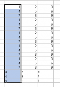
1. Mark the cell range or column you want to manipulate.
2. From the menu “Data->Text To Columns”

 

 

Auto-format of tables

This feature helps you quickly format a table in 1,2,3 clicks without having to go through the details of table border, colors, …etc.

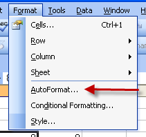
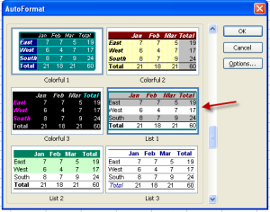
How ? Very simply by clicking on one of the table cells and then the menu “Format->AutoFormat” and select among a set of pre-defined table formats.

 

 

Conditional Formatting

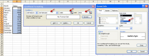
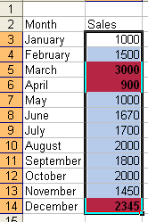
If you are creating automated dashboards and you need to flag out some cells when their values exceeds a certain threshold, then conditional formatting is the tool.

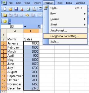
1. click on the cell you need to set a conditional formatting for.
2. Menu “Format–>Conditional Formatting”
3. Adjust the dialogue accordingly.

You can add more  conditions by clicking the “Add >>” button to add more conditional formatting for this range of cells.

You can also delete or modify theses conditional formattings by marking the same range again and recalling the menu “Format–>Conditional Formatting “.

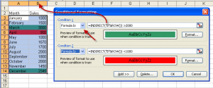
If you want to color a  row according to a certain cell value in in that row, then you need use Conditional Formatting, but you need a workaround using INDIRECT() Function.

 

At the end

There are many more tips and tricks that could help you cut-short most of your daily tasks in Excel. I urge you to learn more about Excel and master this wonderful tool and automate your work with it.

I hope one day I could also write an article about VBA in Excel.

Please comment or rate this article.